Brstjjy

The binomial coefficients can be arranged to form Pascal's triangle, in which each entry is the sum of the two immediately above.

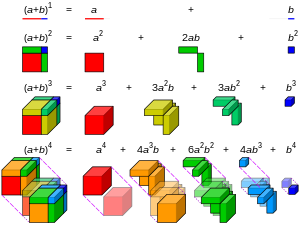
Visualisation of binomial expansion up to the 4th power

In mathematics, any of the positive integers that occurs as a coefficient in the binomial theorem is a binomial coefficient. Commonly, a binomial coefficient is indexed by a pair of integers n ≥ k ≥ 0 and is written (nk).{displaystyle {tbinom {n}{k}}.} It is the coefficient of the x^k term in the polynomial expansion of the binomial power (1 + x)ⁿ, and it is given by the formula

(nk)=n!k!(n−k)!.{displaystyle {binom {n}{k}}={frac {n!}{k!(n-k)!}}.}

For example:

(1+x)4=(40)x0+(41)x1+(42)x2+(43)x3+(44)x4=1+4x+6x2+4x3+x4,{displaystyle {begin{array}{rcl}(1{+}x)^{4}&=&{tbinom {4}{0}}x^{0}+{tbinom {4}{1}}x^{1}+{tbinom {4}{2}}x^{2}+{tbinom {4}{3}}x^{3}+{tbinom {4}{4}}x^{4}\&=&1+4x+6x^{2}+4x^{3}+x^{4},end{array}}}

where (42)=4!2!2!=6{displaystyle {tbinom {4}{2}}={tfrac {4!}{2!2!}}=6}, etc.

Arranging the numbers (n0),(n1),…,(nn){displaystyle {tbinom {n}{0}},{tbinom {n}{1}},ldots ,{tbinom {n}{n}}} in successive rows for n=0,1,2,…{displaystyle n=0,1,2,ldots } gives a triangular array called Pascal's triangle, satisfying the recurrence relation (nk)=(n−1k)+(n−1k−1){displaystyle {tbinom {n}{k}}={tbinom {n-1}{k}}+{tbinom {n-1}{k-1}}}.

The binomial coefficients occur in many areas of mathematics, especially combinatorics.
The symbol (nk){displaystyle {tbinom {n}{k}}} is usually read as "n choose k" because there are (nk){displaystyle {tbinom {n}{k}}} ways to choose an (unordered) subset of k elements from a fixed set of n elements. For example, there are (42)=6{displaystyle {tbinom {4}{2}}=6} ways to choose 2 elements from {1,2,3,4}{displaystyle {1,2,3,4}}, namely {1,2}{displaystyle {1,2}}, {1,3}{displaystyle {1,3}}, {1,4}{displaystyle {1,4}}, {2,3}{displaystyle {2,3}}, {2,4}{displaystyle {2,4}}, {3,4}{displaystyle {3,4}}.

Many properties of (nk){displaystyle {tbinom {n}{k}}} also apply to the generalized binomial coefficients (zk){displaystyle {tbinom {z}{k}}} for any complex number z and integer k ≥ 0.

History and notation

Andreas von Ettingshausen introduced the notation (nk){displaystyle {tbinom {n}{k}}} in 1826,^[1] although the numbers were known centuries earlier (see Pascal's triangle). The earliest known detailed discussion of binomial coefficients is in a tenth-century commentary, by Halayudha, on an ancient Sanskrit text, Pingala's Chandaḥśāstra. In about 1150, the Indian mathematician Bhaskaracharya gave an exposition of binomial coefficients in his book Līlāvatī.^[2]

Alternative notations include C(n, k), _nC_k, ⁿC_k, C^k_n, Cⁿ_k, and C_n,k in all of which the C stands for combinations or choices. Many calculators use variants of the C notation because they can represent it on a single-line display. In this form the binomial coefficients are easily compared to k-permutations of n, written as P(n, k), etc.

Definition and interpretations

For natural numbers (taken to include 0) n and k, the binomial coefficient (nk){displaystyle {tbinom {n}{k}}} can be defined as the coefficient of the monomial X^k in the expansion of (1 + X)ⁿ. The same coefficient also occurs (if k ≤ n) in the binomial formula

(x+y)n=∑k=0n(nk)xn−kyk{displaystyle (x+y)^{n}=sum _{k=0}^{n}{binom {n}{k}}x^{n-k}y^{k}}

(∗)

(valid for any elements x,y of a commutative ring),
which explains the name "binomial coefficient".

Another occurrence of this number is in combinatorics, where it gives the number of ways, disregarding order, that k objects can be chosen from among n objects; more formally, the number of k-element subsets (or k-combinations) of an n-element set. This number can be seen as equal to the one of the first definition, independently of any of the formulas below to compute it: if in each of the n factors of the power (1 + X)ⁿ one temporarily labels the term X with an index i (running from 1 to n), then each subset of k indices gives after expansion a contribution X^k, and the coefficient of that monomial in the result will be the number of such subsets. This shows in particular that (nk){displaystyle {tbinom {n}{k}}} is a natural number for any natural numbers n and k. There are many other combinatorial interpretations of binomial coefficients (counting problems for which the answer is given by a binomial coefficient expression), for instance the number of words formed of n bits (digits 0 or 1) whose sum is k is given by (nk){displaystyle {tbinom {n}{k}}}, while the number of ways to write k=a1+a2+⋯+an{displaystyle k=a_{1}+a_{2}+cdots +a_{n}} where every a_i is a nonnegative integer is given by (n+k−1n−1){displaystyle {tbinom {n+k-1}{n-1}}}. Most of these interpretations are easily seen to be equivalent to counting k-combinations.

Computing the value of binomial coefficients

Several methods exist to compute the value of (nk){displaystyle {tbinom {n}{k}}} without actually expanding a binomial power or counting k-combinations.

Recursive formula

One method uses the recursive, purely additive, formula

(nk)=(n−1k−1)+(n−1k)for all integers n,k:1≤k≤n−1,{displaystyle {binom {n}{k}}={binom {n-1}{k-1}}+{binom {n-1}{k}}quad {text{for all integers }}n,k:1leq kleq n-1,}

with initial/boundary values

(n0)=(nn)=1for all integers n≥0,{displaystyle {binom {n}{0}}={binom {n}{n}}=1quad {text{for all integers }}ngeq 0,}

The formula follows from considering the set {1,2,3,…,n} and counting separately (a) the k-element groupings that include a particular set element, say "i", in every group (since "i" is already chosen to fill one spot in every group, we need only choose k − 1 from the remaining n − 1) and (b) all the k-groupings that don't include "i"; this enumerates all the possible k-combinations of n elements. It also follows from tracing the contributions to X^k in (1 + X)ⁿ⁻¹(1 + X). As there is zero Xⁿ⁺¹ or X⁻¹ in (1 + X)ⁿ, one might extend the definition beyond the above boundaries to include (nk){displaystyle {tbinom {n}{k}}} = 0 when either k > n or k < 0. This recursive formula then allows the construction of Pascal's triangle, surrounded by white spaces where the zeros, or the trivial coefficients, would be.

Multiplicative formula

A more efficient method to compute individual binomial coefficients is given by the formula

(nk)=nk_k!=n(n−1)(n−2)⋯(n−(k−1))k(k−1)(k−2)⋯1=∏i=1kn+1−ii,{displaystyle {binom {n}{k}}={frac {n^{underline {k}}}{k!}}={frac {n(n-1)(n-2)cdots (n-(k-1))}{k(k-1)(k-2)cdots 1}}=prod _{i=1}^{k}{frac {n+1-i}{i}},}

where the numerator of the first fraction nk_{displaystyle n^{underline {k}}} is expressed as a falling factorial power.
This formula is easiest to understand for the combinatorial interpretation of binomial coefficients.
The numerator gives the number of ways to select a sequence of k distinct objects, retaining the order of selection, from a set of n objects. The denominator counts the number of distinct sequences that define the same k-combination when order is disregarded.

Due to the symmetry of the binomial coefficient with regard to k and n−k, calculation may be optimised by setting the upper limit of the product above to the smaller of k and n−k.

Factorial formula

Finally, though computationally unsuitable, there is the compact form, often used in proofs and derivations, which makes repeated use of the familiar factorial function:

(nk)=n!k!(n−k)!for  0≤k≤n,{displaystyle {binom {n}{k}}={frac {n!}{k!,(n-k)!}}quad {text{for }} 0leq kleq n,}

where n! denotes the factorial of n. This formula follows from the multiplicative formula above by multiplying numerator and denominator by (n − k)!; as a consequence it involves many factors common to numerator and denominator. It is less practical for explicit computation (in the case that k is small and n is large) unless common factors are first cancelled (in particular since factorial values grow very rapidly). The formula does exhibit a symmetry that is less evident from the multiplicative formula (though it is from the definitions)

(nk)=(nn−k)for  0≤k≤n,{displaystyle {binom {n}{k}}={binom {n}{n-k}}quad {text{for }} 0leq kleq n,}

(1)

which leads to a more efficient multiplicative computational routine. Using the falling factorial notation,

(nk)={nk_/k!if  k≤n2nn−k_/(n−k)!if  k>n2.{displaystyle {binom {n}{k}}={begin{cases}n^{underline {k}}/k!&{text{if }} kleq {frac {n}{2}}\n^{underline {n-k}}/(n-k)!&{text{if }} k>{frac {n}{2}}end{cases}}.}

Generalization and connection to the binomial series

The multiplicative formula allows the definition of binomial coefficients to be extended^[3] by replacing n by an arbitrary number α (negative, real, complex) or even an element of any commutative ring in which all positive integers are invertible:

(αk)=αk_k!=α(α−1)(α−2)⋯(α−k+1)k(k−1)(k−2)⋯1for k∈N and arbitrary α.{displaystyle {binom {alpha }{k}}={frac {alpha ^{underline {k}}}{k!}}={frac {alpha (alpha -1)(alpha -2)cdots (alpha -k+1)}{k(k-1)(k-2)cdots 1}}quad {text{for }}kin mathbb {N} {text{ and arbitrary }}alpha .}

With this definition one has a generalization of the binomial formula (with one of the variables set to 1), which justifies still calling the (αk){displaystyle {tbinom {alpha }{k}}} binomial coefficients:

(1+X)α=∑k=0∞(αk)Xk.{displaystyle (1+X)^{alpha }=sum _{k=0}^{infty }{alpha choose k}X^{k}.}

(2)

This formula is valid for all complex numbers α and X with |X| < 1. It can also be interpreted as an identity of formal power series in X, where it actually can serve as definition of arbitrary powers of power series with constant coefficient equal to 1; the point is that with this definition all identities hold that one expects for exponentiation, notably

(1+X)α(1+X)β=(1+X)α+βand((1+X)α)β=(1+X)αβ.{displaystyle (1+X)^{alpha }(1+X)^{beta }=(1+X)^{alpha +beta }quad {text{and}}quad ((1+X)^{alpha })^{beta }=(1+X)^{alpha beta }.}

If α is a nonnegative integer n, then all terms with k > n are zero, and the infinite series becomes a finite sum, thereby recovering the binomial formula. However, for other values of α, including negative integers and rational numbers, the series is really infinite.

Pascal's triangle

1000th row of Pascal's triangle, arranged vertically, with grey-scale representations of decimal digits of the coefficients, right-aligned. The left boundary of the image corresponds roughly to the graph of the logarithm of the binomial coefficients, and illustrates that they form a log-concave sequence.

Pascal's rule is the important recurrence relation

(nk)+(nk+1)=(n+1k+1),{displaystyle {n choose k}+{n choose k+1}={n+1 choose k+1},}

(3)

which can be used to prove by mathematical induction that (nk){displaystyle {tbinom {n}{k}}} is a natural number for all n and k, a fact that is not immediately obvious from formula (1).

Pascal's rule also gives rise to Pascal's triangle:

0:									1
1:								1		1
2:							1		2		1
3:						1		3		3		1
4:					1		4		6		4		1
5:				1		5		10		10		5		1
6:			1		6		15		20		15		6		1
7:		1		7		21		35		35		21		7		1
8:	1		8		28		56		70		56		28		8		1

Row number n contains the numbers (nk){displaystyle {tbinom {n}{k}}} for k = 0,…,n. It is constructed by starting with ones at the outside and then always adding two adjacent numbers and writing the sum directly underneath. This method allows the quick calculation of binomial coefficients without the need for fractions or multiplications. For instance, by looking at row number 5 of the triangle, one can quickly read off that

(x + y)⁵ = 1 x⁵ + 5 x⁴y + 10 x³y² + 10 x²y³ + 5 x y⁴ + 1 y⁵.

The differences between elements on other diagonals are the elements in the previous diagonal, as a consequence of the recurrence relation (3) above.

Combinatorics and statistics

Binomial coefficients are of importance in combinatorics, because they provide ready formulas for certain frequent counting problems:

• There are (nk){displaystyle {tbinom {n}{k}}} ways to choose k elements from a set of n elements. See Combination.


• There are (n+k−1k){displaystyle {tbinom {n+k-1}{k}}} ways to choose k elements from a set of n elements if repetitions are allowed. See Multiset.


• There are (n+kk){displaystyle {tbinom {n+k}{k}}} strings containing k ones and n zeros.


• There are (n+1k){displaystyle {tbinom {n+1}{k}}} strings consisting of k ones and n zeros such that no two ones are adjacent.^[4]
  


• The Catalan numbers are 1n+1(2nn).{displaystyle {tfrac {1}{n+1}}{tbinom {2n}{n}}.}
  


• The binomial distribution in statistics is (nk)pk(1−p)n−k.{displaystyle {tbinom {n}{k}}p^{k}(1-p)^{n-k}!.}
  

Binomial coefficients as polynomials

For any nonnegative integer k, the expression (tk){displaystyle scriptstyle {binom {t}{k}}} can be simplified and defined as a polynomial divided by k!:

(tk)=(t)kk!=(t)k(k)k=t(t−1)(t−2)⋯(t−k+1)k(k−1)(k−2)⋯2⋅1;{displaystyle {binom {t}{k}}={frac {(t)_{k}}{k!}}={frac {(t)_{k}}{(k)_{k}}}={frac {t(t-1)(t-2)cdots (t-k+1)}{k(k-1)(k-2)cdots 2cdot 1}};}

this presents a polynomial in t with rational coefficients.

As such, it can be evaluated at any real or complex number t to define binomial coefficients with such first arguments.
These "generalized binomial coefficients" appear in Newton's generalized binomial theorem.

For each k, the polynomial (tk){displaystyle {tbinom {t}{k}}} can be characterized as the unique degree k polynomial p(t) satisfying p(0) = p(1) = ... = p(k − 1) = 0 and p(k) = 1.

Its coefficients are expressible in terms of Stirling numbers of the first kind:

(tk)=∑i=0ks(k,i)tik!.{displaystyle {binom {t}{k}}=sum _{i=0}^{k}s(k,i){frac {t^{i}}{k!}}.}

The derivative of (tk){displaystyle {tbinom {t}{k}}} can be calculated by logarithmic differentiation:

ddt(tk)=(tk)∑i=0k−11t−i.{displaystyle {frac {mathrm {d} }{mathrm {d} t}}{binom {t}{k}}={binom {t}{k}}sum _{i=0}^{k-1}{frac {1}{t-i}},.}

Binomial coefficients as a basis for the space of polynomials

Over any field of characteristic 0 (that is, any field that contains the rational numbers), each polynomial p(t) of degree at most d is uniquely expressible as a linear combination ∑k=0dak(tk){displaystyle sum _{k=0}^{d}a_{k}{binom {t}{k}}} of binomial coefficients. The coefficient a_k is the kth difference of the sequence p(0), p(1), …, p(k).
Explicitly,^[5]

ak=∑i=0k(−1)k−i(ki)p(i).{displaystyle a_{k}=sum _{i=0}^{k}(-1)^{k-i}{binom {k}{i}}p(i).}

(4)

Integer-valued polynomials

Each polynomial (tk){displaystyle {tbinom {t}{k}}} is integer-valued: it has an integer value at all integer inputs t{displaystyle t}.
(One way to prove this is by induction on k, using Pascal's identity.)
Therefore, any integer linear combination of binomial coefficient polynomials is integer-valued too.
Conversely, (4) shows that any integer-valued polynomial is an integer linear combination of these binomial coefficient polynomials.
More generally, for any subring R of a characteristic 0 field K, a polynomial in K[t] takes values in R at all integers if and only if it is an R-linear combination of binomial coefficient polynomials.

Example

The integer-valued polynomial 3t(3t + 1)/2 can be rewritten as

9(t2)+6(t1)+0(t0).{displaystyle 9{tbinom {t}{2}}+6{tbinom {t}{1}}+0{tbinom {t}{0}}.}

Identities involving binomial coefficients

The factorial formula facilitates relating nearby binomial coefficients. For instance, if k is a positive integer and n is arbitrary, then

(nk)=nk(n−1k−1){displaystyle {binom {n}{k}}={frac {n}{k}}{binom {n-1}{k-1}}}

(5)

and, with a little more work,

(n−1k)−(n−1k−1)=n−2kn(nk).{displaystyle {binom {n-1}{k}}-{binom {n-1}{k-1}}={frac {n-2k}{n}}{binom {n}{k}}.}

Moreover, the following may be useful:

(nh)(n−hk)=(nk)(n−kh).{displaystyle {binom {n}{h}}{binom {n-h}{k}}={binom {n}{k}}{binom {n-k}{h}}.}

For constant n, we have the following recurrence:

(nk)=n+1−kk(nk−1).{displaystyle {binom {n}{k}}={frac {n+1-k}{k}}{binom {n}{k-1}}.}

Sums of the binomial coefficients

The formula

∑k=0n(nk)=2n{displaystyle sum _{k=0}^{n}{binom {n}{k}}=2^{n}}

(∗∗)

says the elements in the n^th row of Pascal's triangle always add up to 2 raised to the n^th power. This is obtained from the binomial theorem (∗) by setting x = 1 and y = 1. The formula also has a natural combinatorial interpretation: the left side sums the number of subsets of {1,...,n} of sizes k = 0,1,...,n, giving the total number of subsets. (That is, the left side counts the power set of {1,...,n}.) However, these subsets can also be generated by successively choosing or excluding each element 1,...,n; the n independent binary choices (bit-strings) allow a total of 2n{displaystyle 2^{n}} choices. The left and right sides are two ways to count the same collection of subsets, so they are equal.

The formulas

∑k=0nk(nk)=n2n−1{displaystyle sum _{k=0}^{n}k{binom {n}{k}}=n2^{n-1}}

(6)

and
∑k=0nk2(nk)=(n+n2)2n−2{displaystyle sum _{k=0}^{n}k^{2}{binom {n}{k}}=(n+n^{2})2^{n-2}}
follow from (2) after differentiating with respect to x (twice in the latter) and then substituting x = 1.

The Chu–Vandermonde identity, which holds for any complex-values m and n and any non-negative integer k, is

∑j=0k(mj)(n−mk−j)=(nk){displaystyle sum _{j=0}^{k}{binom {m}{j}}{binom {n-m}{k-j}}={binom {n}{k}}}

(7)

and can be found by examination of the coefficient of xk{displaystyle x^{k}} in the expansion of (1 + x)^m (1 + x)^n − m = (1 + x)ⁿ using equation (2). When m = 1, equation (7) reduces to equation (3). In the special case n = 2m, k = m, using (1), the expansion (7) becomes (as seen in Pascal's triangle at right)

Pascal's triangle, rows 0 through 7. Equation 8 for m = 3 is illustrated in rows 3 and 6 as 12+32+32+12=20.{displaystyle 1^{2}+3^{2}+3^{2}+1^{2}=20.}

∑j=0m(mj)2=(2mm),{displaystyle sum _{j=0}^{m}{binom {m}{j}}^{2}={binom {2m}{m}},}

(8)

where the term on the right side is a central binomial coefficient.

Another form of the Chu–Vandermonde identity, which applies for any integers j, k, and n satisfying 0 ≤ j ≤ k ≤ n, is

∑m=0n(mj)(n−mk−j)=(n+1k+1).{displaystyle sum _{m=0}^{n}{binom {m}{j}}{binom {n-m}{k-j}}={binom {n+1}{k+1}}.}

(9)

The proof is similar, but uses the binomial series expansion (2) with negative integer exponents.
When j = k, equation (9) gives the hockey-stick identity

∑m=kn(mk)=(n+1k+1).{displaystyle sum _{m=k}^{n}{binom {m}{k}}={binom {n+1}{k+1}}.}

Let F(n) denote the n-th Fibonacci number.
Then

∑k=0⌊n/2⌋(n−kk)=F(n+1).{displaystyle sum _{k=0}^{lfloor n/2rfloor }{binom {n-k}{k}}=F(n+1).}

This can be proved by induction using (3) or by Zeckendorf's representation. A combinatorial proof is given below.

Multisections of sums

For integers s and t such that 0≤t<s,{displaystyle 0leq t<s,} series multisection gives the following identity for the sum of binomial coefficients:

(nt)+(nt+s)+(nt+2s)+…=1s∑j=0s−1(2cos⁡πjs)ncos⁡π(n−2t)js.{displaystyle {binom {n}{t}}+{binom {n}{t+s}}+{binom {n}{t+2s}}+ldots ={frac {1}{s}}sum _{j=0}^{s-1}left(2cos {frac {pi j}{s}}right)^{n}cos {frac {pi (n-2t)j}{s}}.}

For small s, these series have particularly nice forms; for example,^[6]

(n0)+(n3)+(n6)+⋯=13(2n+2cos⁡nπ3){displaystyle {binom {n}{0}}+{binom {n}{3}}+{binom {n}{6}}+cdots ={frac {1}{3}}left(2^{n}+2cos {frac {npi }{3}}right)}

(n1)+(n4)+(n7)+⋯=13(2n+2cos⁡(n−2)π3){displaystyle {binom {n}{1}}+{binom {n}{4}}+{binom {n}{7}}+cdots ={frac {1}{3}}left(2^{n}+2cos {frac {(n-2)pi }{3}}right)}

(n2)+(n5)+(n8)+⋯=13(2n+2cos⁡(n−4)π3){displaystyle {binom {n}{2}}+{binom {n}{5}}+{binom {n}{8}}+cdots ={frac {1}{3}}left(2^{n}+2cos {frac {(n-4)pi }{3}}right)}

(n0)+(n4)+(n8)+⋯=12(2n−1+2n2cos⁡nπ4){displaystyle {binom {n}{0}}+{binom {n}{4}}+{binom {n}{8}}+cdots ={frac {1}{2}}left(2^{n-1}+2^{frac {n}{2}}cos {frac {npi }{4}}right)}

(n1)+(n5)+(n9)+⋯=12(2n−1+2n2sin⁡nπ4){displaystyle {binom {n}{1}}+{binom {n}{5}}+{binom {n}{9}}+cdots ={frac {1}{2}}left(2^{n-1}+2^{frac {n}{2}}sin {frac {npi }{4}}right)}

(n2)+(n6)+(n10)+⋯=12(2n−1−2n2cos⁡nπ4){displaystyle {binom {n}{2}}+{binom {n}{6}}+{binom {n}{10}}+cdots ={frac {1}{2}}left(2^{n-1}-2^{frac {n}{2}}cos {frac {npi }{4}}right)}

(n3)+(n7)+(n11)+⋯=12(2n−1−2n2sin⁡nπ4){displaystyle {binom {n}{3}}+{binom {n}{7}}+{binom {n}{11}}+cdots ={frac {1}{2}}left(2^{n-1}-2^{frac {n}{2}}sin {frac {npi }{4}}right)}

Partial sums

Although there is no closed formula for partial sums

∑j=0k(nj){displaystyle sum _{j=0}^{k}{binom {n}{j}}}

of binomial coefficients,^[7] one can again use (3) and induction to show that for k = 0, ..., n − 1,

∑j=0k(−1)j(nj)=(−1)k(n−1k){displaystyle sum _{j=0}^{k}(-1)^{j}{binom {n}{j}}=(-1)^{k}{binom {n-1}{k}}},

with special case^[8]

∑j=0n(−1)j(nj)=0{displaystyle sum _{j=0}^{n}(-1)^{j}{binom {n}{j}}=0}

for n > 0. This latter result is also a special case of the result from the theory of finite differences that for any polynomial P(x) of degree less than n,^[9]

∑j=0n(−1)j(nj)P(j)=0.{displaystyle sum _{j=0}^{n}(-1)^{j}{binom {n}{j}}P(j)=0.}

Differentiating (2) k times and setting x = −1 yields this for
P(x)=x(x−1)⋯(x−k+1){displaystyle P(x)=x(x-1)cdots (x-k+1)},
when 0 ≤ k < n,
and the general case follows by taking linear combinations of these.

When P(x) is of degree less than or equal to n,

∑j=0n(−1)j(nj)P(n−j)=n!an{displaystyle sum _{j=0}^{n}(-1)^{j}{binom {n}{j}}P(n-j)=n!a_{n}}

(10)

where an{displaystyle a_{n}} is the coefficient of degree n in P(x).

More generally for (10),

∑j=0n(−1)j(nj)P(m+(n−j)d)=dnn!an{displaystyle sum _{j=0}^{n}(-1)^{j}{binom {n}{j}}P(m+(n-j)d)=d^{n}n!a_{n}}

where m and d are complex numbers. This follows immediately applying (10) to the polynomial Q(x):=P(m + dx) instead of P(x), and observing that Q(x) has still degree less than or equal to n, and that its coefficient of degree n is dⁿa_n.

The series
k−1k∑j=0∞1(j+xk)=1(x−1k−1){displaystyle {frac {k-1}{k}}sum _{j=0}^{infty }{frac {1}{binom {j+x}{k}}}={frac {1}{binom {x-1}{k-1}}}} is convergent for k ≥ 2. This formula is used in the analysis of the German tank problem. It follows from k−1k∑j=0M1(j+xk)=1(x−1k−1)−1(M+xk−1){displaystyle {frac {k-1}{k}}sum _{j=0}^{M}{frac {1}{binom {j+x}{k}}}={frac {1}{binom {x-1}{k-1}}}-{frac {1}{binom {M+x}{k-1}}}}
which is proved by induction on M.

Identities with combinatorial proofs

Many identities involving binomial coefficients can be proved by combinatorial means. For example, for nonnegative integers n≥q{displaystyle {n}geq {q}}, the identity

∑k=qn(nk)(kq)=2n−q(nq){displaystyle sum _{k=q}^{n}{binom {n}{k}}{binom {k}{q}}=2^{n-q}{binom {n}{q}}}

(which reduces to (6) when q = 1) can be given a double counting proof, as follows. The left side counts the number of ways of selecting a subset of [n] = {1, 2, …, n} with at least q elements, and marking q elements among those selected. The right side counts the same thing, because there are (nq){displaystyle {tbinom {n}{q}}} ways of choosing a set of q elements to mark, and 2n−q{displaystyle 2^{n-q}} to choose which of the remaining elements of [n] also belong to the subset.

In Pascal's identity

(nk)=(n−1k−1)+(n−1k),{displaystyle {n choose k}={n-1 choose k-1}+{n-1 choose k},}

both sides count the number of k-element subsets of [n]: the two terms on the right side group them into those that contain element n and those that do not.

The identity (8) also has a combinatorial proof. The identity reads

∑k=0n(nk)2=(2nn).{displaystyle sum _{k=0}^{n}{binom {n}{k}}^{2}={binom {2n}{n}}.}

Suppose you have 2n{displaystyle 2n} empty squares arranged in a row and you want to mark (select) n of them. There are (2nn){displaystyle {tbinom {2n}{n}}} ways to do this. On the other hand, you may select your n squares by selecting k squares from among the first n and n−k{displaystyle n-k} squares from the remaining n squares; any k from 0 to n will work. This gives

∑k=0n(nk)(nn−k)=(2nn).{displaystyle sum _{k=0}^{n}{binom {n}{k}}{binom {n}{n-k}}={binom {2n}{n}}.}

Now apply (5) to get the result.

If one denotes by F(i) the sequence of Fibonacci numbers, indexed so that F(0) = F(1) = 1, then the identity

∑k=0⌊n2⌋(n−kk)=F(n){displaystyle sum _{k=0}^{lfloor {frac {n}{2}}rfloor }{tbinom {n-k}{k}}=F(n)}

(n−kk){displaystyle {tbinom {n-k}{k}}}

Sum of coefficients row

The number of k-combinations for all k, ∑0≤k≤n(nk)=2n{displaystyle sum _{0leq {k}leq {n}}{binom {n}{k}}=2^{n}}, is the sum of the nth row (counting from 0) of the binomial coefficients. These combinations are enumerated by the 1 digits of the set of base 2 numbers counting from 0 to 2n−1{displaystyle 2^{n}-1}, where each digit position is an item from the set of n.

Dixon's identity

Dixon's identity is

∑k=−aa(−1)k(2ak+a)3=(3a)!(a!)3{displaystyle sum _{k=-a}^{a}(-1)^{k}{2a choose k+a}^{3}={frac {(3a)!}{(a!)^{3}}}}

or, more generally,

∑k=−aa(−1)k(a+ba+k)(b+cb+k)(c+ac+k)=(a+b+c)!a!b!c!,{displaystyle sum _{k=-a}^{a}(-1)^{k}{a+b choose a+k}{b+c choose b+k}{c+a choose c+k}={frac {(a+b+c)!}{a!,b!,c!}},,}

where a, b, and c are non-negative integers.

Continuous identities

Certain trigonometric integrals have values expressible in terms of
binomial coefficients:

For m,n∈N{displaystyle textstyle m,nin mathbb {N} }

∫−ππcos⁡((2m−n)x)cosn⁡x dx=π2n−1(nm){displaystyle int _{-pi }^{pi }cos((2m-n)x)cos ^{n}x dx={frac {pi }{2^{n-1}}}{binom {n}{m}}}

∫−ππsin⁡((2m−n)x)sinn⁡x dx={(−1)m+(n+1)/2π2n−1(nm)n odd0otherwise{displaystyle int _{-pi }^{pi }sin((2m-n)x)sin ^{n}x dx=left{{begin{array}{cc}(-1)^{m+(n+1)/2}{frac {pi }{2^{n-1}}}{binom {n}{m}}&n{text{ odd}}\0&{text{otherwise}}\end{array}}right.}

∫−ππcos⁡((2m−n)x)sinn⁡x dx={(−1)m+(n/2)π2n−1(nm)n even0otherwise{displaystyle int _{-pi }^{pi }cos((2m-n)x)sin ^{n}x dx=left{{begin{array}{cc}(-1)^{m+(n/2)}{frac {pi }{2^{n-1}}}{binom {n}{m}}&n{text{ even}}\0&{text{otherwise}}\end{array}}right.}

These can be proved by using Euler's formula to convert trigonometric functions to complex exponentials, expanding using the binomial theorem, and integrating term by term.

Generating functions

Ordinary generating functions

For a fixed n, the ordinary generating function of the sequence (n0),(n1),(n2),…{displaystyle {tbinom {n}{0}},{tbinom {n}{1}},{tbinom {n}{2}},ldots } is

∑k=0∞(nk)xk=(1+x)n.{displaystyle sum _{k=0}^{infty }{n choose k}x^{k}=(1+x)^{n}.}

For a fixed k, the ordinary generating function of the sequence (0k),(1k),(2k),…,{displaystyle {tbinom {0}{k}},{tbinom {1}{k}},{tbinom {2}{k}},ldots ,} is

∑n=k∞(nk)yn=yk(1−y)k+1.{displaystyle sum _{n=k}^{infty }{n choose k}y^{n}={frac {y^{k}}{(1-y)^{k+1}}}.}

The bivariate generating function of the binomial coefficients is

∑n=0∞∑k=0n(nk)xkyn=11−y−xy.{displaystyle sum _{n=0}^{infty }sum _{k=0}^{n}{n choose k}x^{k}y^{n}={frac {1}{1-y-xy}}.}

Another, symmetric, bivariate generating function of the binomial coefficients is

∑n=0∞∑k=0∞(n+kk)xkyn=11−x−y.{displaystyle sum _{n=0}^{infty }sum _{k=0}^{infty }{n+k choose k}x^{k}y^{n}={frac {1}{1-x-y}}.}

Exponential generating function

A symmetric exponential bivariate generating function of the binomial coefficients is:

∑n=0∞∑k=0∞(n+kk)xkyn(n+k)!=ex+y.{displaystyle sum _{n=0}^{infty }sum _{k=0}^{infty }{n+k choose k}{frac {x^{k}y^{n}}{(n+k)!}}=e^{x+y}.}

Divisibility properties

In 1852, Kummer proved that if m and n are nonnegative integers and p is a prime number, then the largest power of p dividing (m+nm){displaystyle {tbinom {m+n}{m}}} equals p^c, where c is the number of carries when m and n are added in base p.
Equivalently, the exponent of a prime p in (nk){displaystyle {tbinom {n}{k}}}
equals the number of nonnegative integers j such that the fractional part of k/p^j is greater than the fractional part of n/p^j. It can be deduced from this that (nk){displaystyle {tbinom {n}{k}}} is divisible by n/gcd(n,k). In particular therefore it follows that p divides (prs){displaystyle {tbinom {p^{r}}{s}}} for all positive integers r and s such that s < p^r. However this is not true of higher powers of p: for example 9 does not divide (96){displaystyle {tbinom {9}{6}}}.

A somewhat surprising result by David Singmaster (1974) is that any integer divides almost all binomial coefficients. More precisely, fix an integer d and let f(N) denote the number of binomial coefficients (nk){displaystyle {tbinom {n}{k}}} with n < N such that d divides (nk){displaystyle {tbinom {n}{k}}}. Then

limN→∞f(N)N(N+1)/2=1.{displaystyle lim _{Nto infty }{frac {f(N)}{N(N+1)/2}}=1.}

Since the number of binomial coefficients (nk){displaystyle {tbinom {n}{k}}} with n < N is N(N + 1) / 2, this implies that the density of binomial coefficients divisible by d goes to 1.

Binomial coefficients have divisibility properties related to least common multiples of consecutive integers. For example:^[11]

(n+kk){displaystyle {binom {n+k}{k}}} divides lcm(n,n+1,…,n+k)n{displaystyle {frac {{text{lcm}}(n,n+1,ldots ,n+k)}{n}}}.

(n+kk){displaystyle {binom {n+k}{k}}} is a multiple of lcm(n,n+1,…,n+k)n⋅lcm((k0),(k1),…,(kk)){displaystyle {frac {{text{lcm}}(n,n+1,ldots ,n+k)}{ncdot {text{lcm}}({binom {k}{0}},{binom {k}{1}},ldots ,{binom {k}{k}})}}}.

Another fact:
An integer n ≥ 2 is prime if and only if
all the intermediate binomial coefficients

(n1),(n2),…,(nn−1){displaystyle {binom {n}{1}},{binom {n}{2}},ldots ,{binom {n}{n-1}}}

are divisible by n.

Proof:
When p is prime, p divides

(pk)=p⋅(p−1)⋯(p−k+1)k⋅(k−1)⋯1{displaystyle {binom {p}{k}}={frac {pcdot (p-1)cdots (p-k+1)}{kcdot (k-1)cdots 1}}} for all 0 < k < p

because (pk){displaystyle {tbinom {p}{k}}} is a natural number and p divides the numerator but not the denominator.
When n is composite, let p be the smallest prime factor of n and let k = n/p. Then 0 < p < n and

(np)=n(n−1)(n−2)⋯(n−p+1)p!=k(n−1)(n−2)⋯(n−p+1)(p−1)!≢0(modn){displaystyle {binom {n}{p}}={frac {n(n-1)(n-2)cdots (n-p+1)}{p!}}={frac {k(n-1)(n-2)cdots (n-p+1)}{(p-1)!}}not equiv 0{pmod {n}}}

otherwise the numerator k(n − 1)(n − 2)×...×(n − p + 1) has to be divisible by n = k×p, this can only be the case when (n − 1)(n − 2)×...×(n − p + 1) is divisible by p. But n is divisible by p, so p does not divide n − 1, n − 2, ..., n − p + 1 and because p is prime, we know that p does not divide (n − 1)(n − 2)×...×(n − p + 1) and so the numerator cannot be divisible by n.

Bounds and asymptotic formulas

The following bounds for (nk){displaystyle {tbinom {n}{k}}} hold for all values of n and k such that 1 ≤ k ≤ n:

nkkk≤(nk)≤nkk!<(n⋅ek)k{displaystyle {frac {n^{k}}{k^{k}}}leq {n choose k}leq {frac {n^{k}}{k!}}<left({frac {ncdot e}{k}}right)^{k}}.

The first inequality follows from the fact that (nk)=nk⋅n−1k−1⋯n−(k−1)1{displaystyle {n choose k}={frac {n}{k}}cdot {frac {n-1}{k-1}}cdots {frac {n-(k-1)}{1}}} and each of these k{displaystyle k} terms in this product is ≥nk{displaystyle geq {frac {n}{k}}}. A similar argument can be made to show (nk)≤nkk!{displaystyle {n choose k}leq {frac {n^{k}}{k!}}}. The final strict inequality follows from multiplying (nk)k{displaystyle left({frac {n}{k}}right)^{k}} by the Taylor series for ek{displaystyle e^{k}}.

From the divisibility properties we can infer that

lcm(n−k,…,n)(n−k)⋅lcm((k0),…,(kk))≤(nk)≤lcm(n−k,…,n)n−k{displaystyle {frac {{text{lcm}}(n-k,ldots ,n)}{(n-k)cdot {text{lcm}}({binom {k}{0}},ldots ,{binom {k}{k}})}}leq {binom {n}{k}}leq {frac {{text{lcm}}(n-k,ldots ,n)}{n-k}}},

where both equalities can be achieved.^[11]

Stirling's approximation yields the following approximation, when n,i{displaystyle n,i} are sufficiently large:

(ni)∼n2πi(n−i)⋅nnii(n−i)n−i{displaystyle {n choose i}sim {sqrt {n over 2pi i(n-i)}}cdot {n^{n} over i^{i}(n-i)^{n-i}}}

In particular, when n{displaystyle n} is sufficiently large:

(2nn)∼4nπn{displaystyle {2n choose n}sim {frac {4^{n}}{sqrt {pi n}}}}

Also:^[why?]

n(2nn)≥22n−1{displaystyle {sqrt {n}}{2n choose n}geq 2^{2n-1}} and, in general, n(mnn)≥mm(n−1)+1(m−1)(m−1)(n−1){displaystyle {sqrt {n}}{mn choose n}geq {frac {m^{m(n-1)+1}}{(m-1)^{(m-1)(n-1)}}}} for m ≥ 2 and n ≥ 1,

For k{displaystyle k} and n−k{displaystyle n-k} both much larger than 1, Stirling's approximation also yields the following asymptotic approximation:

log2⁡(nk)∼nH(k/n)=nlog2⁡(n/k)+(n−k)log2⁡(n/(n−k)){displaystyle log _{2}{n choose k}sim nH(k/n)=nlog _{2}(n/k)+(n-k)log _{2}(n/(n-k))}

where H(ϵ)=−ϵlog2⁡(ϵ)−(1−ϵ)log2⁡(1−ϵ){displaystyle H(epsilon )=-epsilon log _{2}(epsilon )-(1-epsilon )log _{2}(1-epsilon )} is the binary entropy of ϵ{displaystyle epsilon }.
More precisely, for all integers n≥k≥1{displaystyle ngeq kgeq 1} with ϵ≐k/n≤1/2{displaystyle epsilon doteq k/nleq 1/2}, we can estimate the sum of the first k+1{displaystyle k+1} binomial coefficients as follows:^[12]

18nϵ(1−ϵ)⋅2H(ϵ)⋅n≤∑i=0k(ni)≤2H(ϵ)⋅n.{displaystyle {frac {1}{sqrt {8nepsilon (1-epsilon )}}}cdot 2^{H(epsilon )cdot n}leq sum _{i=0}^{k}{binom {n}{i}}leq 2^{H(epsilon )cdot n},.}

When n{displaystyle n} is large and k{displaystyle k} is much smaller than n{displaystyle n}, one can also write

(nk)=n(n−1)…(n−k+1)k!≈(n−k/2)kkke−k2πk=(n/k−0.5)kek2πk,{displaystyle {n choose k}={frac {n(n-1)dots (n-k+1)}{k!}}approx {frac {(n-k/2)^{k}}{k^{k}e^{-k}{sqrt {2pi k}}}}={frac {(n/k-0.5)^{k}e^{k}}{sqrt {2pi k}}},,}

and therefore

ln⁡(nk)≈kln⁡(n/k−0.5)+k−0.5ln⁡(2πk).{displaystyle ln {n choose k}approx kln(n/k-0.5)+k-0.5ln(2pi k),.}

If more precision is desired, one can approximate ln⁡(n(n−1)…(n−k+1)){displaystyle ln {(n(n-1)dots (n-k+1))}} with an integral, obtaining

ln⁡(nk)≈(n+0.5)ln⁡n+0.5n−k+0.5+kln⁡n−k+0.5k−0.5ln⁡(2πk){displaystyle ln {n choose k}approx (n+0.5)ln {frac {n+0.5}{n-k+0.5}}+kln {frac {n-k+0.5}{k}}-0.5ln(2pi k)}

For n=20{displaystyle n=20} and k=10{displaystyle k=10}, ln⁡(nk)≈12.127{displaystyle ln {tbinom {n}{k}}approx 12.127}, and these approximations yield 12.312 and 12.133 respectively.

The infinite product formula (cf. Gamma function, alternative definition)

(−1)k(zk)=(−z+k−1k)=1Γ(−z)1(k+1)z+1∏j=k+1(1+1j)−z−11−z+1j{displaystyle (-1)^{k}{z choose k}={-z+k-1 choose k}={frac {1}{Gamma (-z)}}{frac {1}{(k+1)^{z+1}}}prod _{j=k+1}{frac {(1+{frac {1}{j}})^{-z-1}}{1-{frac {z+1}{j}}}}}

yields the asymptotic formulas

(zk)≈(−1)kΓ(−z)kz+1and(z+kk)=kzΓ(z+1)(1+z(z+1)2k+O(k−2)){displaystyle {z choose k}approx {frac {(-1)^{k}}{Gamma (-z)k^{z+1}}}qquad mathrm {and} qquad {z+k choose k}={frac {k^{z}}{Gamma (z+1)}}left(1+{frac {z(z+1)}{2k}}+{mathcal {O}}left(k^{-2}right)right)}

as k→∞{displaystyle kto infty }.

This asymptotic behaviour is contained in the approximation

(z+kk)≈ez(Hk−γ)Γ(z+1){displaystyle {z+k choose k}approx {frac {e^{z(H_{k}-gamma )}}{Gamma (z+1)}}}

as well. (Here Hk{displaystyle H_{k}} is the k-th harmonic number and γ{displaystyle gamma } is the Euler–Mascheroni constant.)

Further, the asymptotic formula

(z+kj)(kj)→(1−jk)−zand(jj−k)(j−zj−k)→(jk)z{displaystyle {frac {z+k choose j}{k choose j}}to left(1-{frac {j}{k}}right)^{-z}quad {text{and}}quad {frac {j choose j-k}{j-z choose j-k}}to left({frac {j}{k}}right)^{z}}

hold true, whenever k→∞{displaystyle kto infty } and j/k→x{displaystyle j/kto x} for some complex number x{displaystyle x}.

A simple and rough upper bound for the sum of binomial coefficients can be obtained using the binomial theorem:

∑i=0k(ni)≤∑i=0kni⋅1k−i≤(1+n)k{displaystyle sum _{i=0}^{k}{n choose i}leq sum _{i=0}^{k}n^{i}cdot 1^{k-i}leq (1+n)^{k}}

If n is large and k is linear in n, various precise asymptotic estimates exist for the binomial coefficient (nk){displaystyle {binom {n}{k}}}. For example, if |n/2−k|=o(n2/3){displaystyle |n/2-k|=o(n^{2/3})} then^[13]

(nk)∼(nn2)e−d2/(2n)∼2n12nπe−d2/(2n){displaystyle {binom {n}{k}}sim {binom {n}{frac {n}{2}}}e^{-d^{2}/(2n)}sim {frac {2^{n}}{sqrt {{frac {1}{2}}npi }}}e^{-d^{2}/(2n)}}

where d = n − 2k.

Generalizations

Generalization to multinomials

Binomial coefficients can be generalized to multinomial coefficients defined to be the number:

(nk1,k2,…,kr)=n!k1!k2!⋯kr!{displaystyle {n choose k_{1},k_{2},ldots ,k_{r}}={frac {n!}{k_{1}!k_{2}!cdots k_{r}!}}}

where

∑i=1rki=n.{displaystyle sum _{i=1}^{r}k_{i}=n.}

While the binomial coefficients represent the coefficients of (x+y)ⁿ, the multinomial coefficients
represent the coefficients of the polynomial

(x1+x2+⋯+xr)n.{displaystyle (x_{1}+x_{2}+cdots +x_{r})^{n}.}

The case r = 2 gives binomial coefficients:

(nk1,k2)=(nk1,n−k1)=(nk1)=(nk2).{displaystyle {n choose k_{1},k_{2}}={n choose k_{1},n-k_{1}}={n choose k_{1}}={n choose k_{2}}.}

The combinatorial interpretation of multinomial coefficients is distribution of n distinguishable elements over r (distinguishable) containers, each containing exactly k_i elements, where i is the index of the container.

Multinomial coefficients have many properties similar to those of binomial coefficients, for example the recurrence relation:

(nk1,k2,…,kr)=(n−1k1−1,k2,…,kr)+(n−1k1,k2−1,…,kr)+…+(n−1k1,k2,…,kr−1){displaystyle {n choose k_{1},k_{2},ldots ,k_{r}}={n-1 choose k_{1}-1,k_{2},ldots ,k_{r}}+{n-1 choose k_{1},k_{2}-1,ldots ,k_{r}}+ldots +{n-1 choose k_{1},k_{2},ldots ,k_{r}-1}}

and symmetry:

(nk1,k2,…,kr)=(nkσ1,kσ2,…,kσr){displaystyle {n choose k_{1},k_{2},ldots ,k_{r}}={n choose k_{sigma _{1}},k_{sigma _{2}},ldots ,k_{sigma _{r}}}}

where (σi){displaystyle (sigma _{i})} is a permutation of (1,2,...,r).

Taylor series

Using Stirling numbers of the first kind the series expansion around any arbitrarily chosen point z0{displaystyle z_{0}} is

(zk)=1k!∑i=0kzisk,i=∑i=0k(z−z0)i∑j=ik(z0j−i)sk+i−j,i(k+i−j)!=∑i=0k(z−z0)i∑j=ikz0j−i(ji)sk,jk!.{displaystyle {begin{aligned}{z choose k}={frac {1}{k!}}sum _{i=0}^{k}z^{i}s_{k,i}&=sum _{i=0}^{k}(z-z_{0})^{i}sum _{j=i}^{k}{z_{0} choose j-i}{frac {s_{k+i-j,i}}{(k+i-j)!}}\&=sum _{i=0}^{k}(z-z_{0})^{i}sum _{j=i}^{k}z_{0}^{j-i}{j choose i}{frac {s_{k,j}}{k!}}.end{aligned}}}

Binomial coefficient with n = 1/2

The definition of the binomial coefficients can be extended to the case where n{displaystyle n} is real and k{displaystyle k} is integer.

In particular, the following identity holds for any non-negative integer k{displaystyle k} :

(1/2k)=(2kk)(−1)k+122k(2k−1).{displaystyle {{1/2} choose {k}}={{2k} choose {k}}{frac {(-1)^{k+1}}{2^{2k}(2k-1)}}.}

This shows up when expanding 1+x{displaystyle {sqrt {1+x}}} into a power series using the Newton binomial series :

1+x=∑k≥0(1/2k)xk.{displaystyle {sqrt {1+x}}=sum _{kgeq 0}{binom {1/2}{k}}x^{k}.}

Identity for the product of binomial coefficients

One can express the product of binomial coefficients as a linear combination of binomial coefficients:

(zm)(zn)=∑k=0m(m+n−kk,m−k,n−k)(zm+n−k),{displaystyle {z choose m}{z choose n}=sum _{k=0}^{m}{m+n-k choose k,m-k,n-k}{z choose m+n-k},}

where the connection coefficients are multinomial coefficients. In terms of labelled combinatorial objects, the connection coefficients represent the number of ways to assign m + n − k labels to a pair of labelled combinatorial objects—of weight m and n respectively—that have had their first k labels identified, or glued together to get a new labelled combinatorial object of weight m + n − k. (That is, to separate the labels into three portions to apply to the glued part, the unglued part of the first object, and the unglued part of the second object.) In this regard, binomial coefficients are to exponential generating series what falling factorials are to ordinary generating series.

Partial fraction decomposition

The partial fraction decomposition of the reciprocal is given by

1(zn)=∑i=0n−1(−1)n−1−i(ni)n−iz−i,1(z+nn)=∑i=1n(−1)i−1(ni)iz+i.{displaystyle {frac {1}{z choose n}}=sum _{i=0}^{n-1}(-1)^{n-1-i}{n choose i}{frac {n-i}{z-i}},qquad {frac {1}{z+n choose n}}=sum _{i=1}^{n}(-1)^{i-1}{n choose i}{frac {i}{z+i}}.}

Newton's binomial series

Newton's binomial series, named after Sir Isaac Newton, is a generalization of the binomial theorem to infinite series:

(1+z)α=∑n=0∞(αn)zn=1+(α1)z+(α2)z2+⋯.{displaystyle (1+z)^{alpha }=sum _{n=0}^{infty }{alpha choose n}z^{n}=1+{alpha choose 1}z+{alpha choose 2}z^{2}+cdots .}

The identity can be obtained by showing that both sides satisfy the differential equation (1 + z) f'(z) = α f(z).

The radius of convergence of this series is 1. An alternative expression is

1(1−z)α+1=∑n=0∞(n+αn)zn{displaystyle {frac {1}{(1-z)^{alpha +1}}}=sum _{n=0}^{infty }{n+alpha choose n}z^{n}}

where the identity

(nk)=(−1)k(k−n−1k){displaystyle {n choose k}=(-1)^{k}{k-n-1 choose k}}

is applied.

Multiset (rising) binomial coefficient

Binomial coefficients count subsets of prescribed size from a given set. A related combinatorial problem is to count multisets of prescribed size with elements drawn from a given set, that is, to count the number of ways to select a certain number of elements from a given set with the possibility of selecting the same element repeatedly. The resulting numbers are called multiset coefficients;^[14] the number of ways to "multichoose" (i.e., choose with replacement) k items from an n element set is denoted ((nk)){displaystyle left(!!{binom {n}{k}}!!right)}.

To avoid ambiguity and confusion with n's main denotation in this article,
let f = n = r + (k – 1) and r = f – (k – 1).

Multiset coefficients may be expressed in terms of binomial coefficients by the rule

(fk)=((rk))=(r+k−1k).{displaystyle {binom {f}{k}}=left(!!{binom {r}{k}}!!right)={binom {r+k-1}{k}}.}

One possible alternative characterization of this identity is as follows:
We may define the falling factorial as

(f)k=fk_=(f−k+1)⋯(f−3)⋅(f−2)⋅(f−1)⋅f{displaystyle (f)_{k}=f^{underline {k}}=(f-k+1)cdots (f-3)cdot (f-2)cdot (f-1)cdot f},

and the corresponding rising factorial as

|r(k)=rk¯=r⋅(r+1)⋅(r+2)⋅(r+3)⋯(r+k−1){displaystyle {color {white}{big |}}r^{(k)}=,r^{overline {k}}=,rcdot (r+1)cdot (r+2)cdot (r+3)cdots (r+k-1)};

so, for example,

17⋅18⋅19⋅20⋅21=(21)5=215_=175¯=17(5){displaystyle 17cdot 18cdot 19cdot 20cdot 21=(21)_{5}=21^{underline {5}}=17^{overline {5}}=17^{(5)}}.

Then the binomial coefficients may be written as

(fk)=(f)kk!=(f−k+1)⋯(f−2)⋅(f−1)⋅f1⋅2⋅3⋅4⋅5⋯k{displaystyle {binom {f}{k}}={frac {(f)_{k}}{k!}}={frac {(f-k+1)cdots (f-2)cdot (f-1)cdot f}{1cdot 2cdot 3cdot 4cdot 5cdots k}}},

while the corresponding multiset coefficient is defined by replacing the falling with the rising factorial:

((rk))=r(k)k!=r⋅(r+1)⋅(r+2)⋯(r+k−1)1⋅2⋅3⋅4⋅5⋯k{displaystyle left(!!{binom {r}{k}}!!right)={frac {r^{(k)}}{k!}}={frac {rcdot (r+1)cdot (r+2)cdots (r+k-1)}{1cdot 2cdot 3cdot 4cdot 5cdots k}}}.

Generalization to negative integers

For any n,

(−nk)=−n⋅−(n+1)⋯−(n+k−2)⋅−(n+k−1)k!=(−1)kn⋅(n+1)⋅(n+2)⋯(n+k−1)k!=(−1)k(n+k−1k)=(−1)k((nk)).{displaystyle {begin{aligned}{binom {-n}{k}}&={frac {-ncdot -(n+1)dots -(n+k-2)cdot -(n+k-1)}{k!}}\&=(-1)^{k};{frac {ncdot (n+1)cdot (n+2)cdots (n+k-1)}{k!}}\&=(-1)^{k}{binom {n+k-1}{k}}\&=(-1)^{k}left(!!{binom {n}{k}}!!right);.end{aligned}}}

In particular, binomial coefficients evaluated at negative integers are given by signed multiset coefficients. In the special case n=−1{displaystyle n=-1}, this reduces to (−1)k=(−1k)=((−kk)).{displaystyle (-1)^{k}={binom {-1}{k}}=left(!!{binom {-k}{k}}!!right),.}

For example, if n = -4 and k = 7, then r = 4 and f = 10:

(−47)=−10⋅−9⋅−8⋅−7⋅−6⋅−5⋅−41⋅2⋅3⋅4⋅5⋅6⋅7=(−1)74⋅5⋅6⋅7⋅8⋅9⋅101⋅2⋅3⋅4⋅5⋅6⋅7=((−77))((47))=(−17)(107).{displaystyle {begin{aligned}{binom {-4}{7}}&={frac {-10cdot -9cdot -8cdot -7cdot -6cdot -5cdot -4}{1cdot 2cdot 3cdot 4cdot 5cdot 6cdot 7}}\&=(-1)^{7};{frac {4cdot 5cdot 6cdot 7cdot 8cdot 9cdot 10}{1cdot 2cdot 3cdot 4cdot 5cdot 6cdot 7}}\&=left(!!{binom {-7}{7}}!!right)left(!!{binom {4}{7}}!!right)={binom {-1}{7}}{binom {10}{7}}.end{aligned}}}

Two real or complex valued arguments

The binomial coefficient is generalized to two real or complex valued arguments using the gamma function or beta function via

(xy)=Γ(x+1)Γ(y+1)Γ(x−y+1)=1(x+1)B(x−y+1,y+1).{displaystyle {x choose y}={frac {Gamma (x+1)}{Gamma (y+1)Gamma (x-y+1)}}={frac {1}{(x+1)mathrm {B} (x-y+1,y+1)}}.}

This definition inherits these following additional properties from Γ{displaystyle Gamma }:

(xy)=sin⁡(yπ)sin⁡(xπ)(−y−1−x−1)=sin⁡((x−y)π)sin⁡(xπ)(y−x−1y);{displaystyle {x choose y}={frac {sin(ypi )}{sin(xpi )}}{-y-1 choose -x-1}={frac {sin((x-y)pi )}{sin(xpi )}}{y-x-1 choose y};}

moreover,

(xy)⋅(yx)=sin⁡((x−y)π)(x−y)π.{displaystyle {x choose y}cdot {y choose x}={frac {sin((x-y)pi )}{(x-y)pi }}.}

The resulting function has been little-studied, apparently first being graphed in (Fowler 1996). Notably, many binomial identities fail: (nm)=(nn−m){displaystyle textstyle {{n choose m}={n choose n-m}}} but (−nm)≠(−n−n−m){displaystyle textstyle {{-n choose m}neq {-n choose -n-m}}} for n positive (so −n{displaystyle -n} negative). The behavior is quite complex, and markedly different in various octants (that is, with respect to the x and y axes and the line y=x{displaystyle y=x}), with the behavior for negative x having singularities at negative integer values and a checkerboard of positive and negative regions:

• in the octant 0≤y≤x{displaystyle 0leq yleq x} it is a smoothly interpolated form of the usual binomial, with a ridge ("Pascal's ridge").


• in the octant 0≤x≤y{displaystyle 0leq xleq y} and in the quadrant x≥0,y≤0{displaystyle xgeq 0,yleq 0} the function is close to zero.


• in the quadrant x≤0,y≥0{displaystyle xleq 0,ygeq 0} the function is alternatingly very large positive and negative on the parallelograms with vertices

(−n,m+1),(−n,m),(−n−1,m−1),(−n−1,m){displaystyle (-n,m+1),(-n,m),(-n-1,m-1),(-n-1,m)}

• in the octant 0>x>y{displaystyle 0>x>y} the behavior is again alternatingly very large positive and negative, but on a square grid.


• in the octant −1>y>x+1{displaystyle -1>y>x+1} it is close to zero, except for near the singularities.

Generalization to q-series

The binomial coefficient has a q-analog generalization known as the Gaussian binomial coefficient.

Generalization to infinite cardinals

The definition of the binomial coefficient can be generalized to infinite cardinals by defining:

(αβ)=|{B⊆A:|B|=β}|{displaystyle {alpha choose beta }=|{Bsubseteq A:|B|=beta }|}

where A is some set with cardinality α{displaystyle alpha }. One can show that the generalized binomial coefficient is well-defined, in the sense that no matter what set we choose to represent the cardinal number α{displaystyle alpha }, (αβ){displaystyle {alpha choose beta }} will remain the same. For finite cardinals, this definition coincides with the standard definition of the binomial coefficient.

Assuming the Axiom of Choice, one can show that (αα)=2α{displaystyle {alpha choose alpha }=2^{alpha }} for any infinite cardinal α{displaystyle alpha }.

Binomial coefficient in programming languages

The notation (nk){displaystyle {n choose k}} is convenient in handwriting but inconvenient for typewriters and computer terminals. Many programming languages do not offer a standard subroutine for computing the binomial coefficient, but for example both the APL programming language and the (related) J programming language use the exclamation mark: k ! n .

Naive implementations of the factorial formula, such as the following snippet in Python:

from math import factorial

def binomialCoefficient(n, k):

    return factorial(n) // (factorial(k) * factorial(n - k))

are very slow and are useless for calculating factorials of very high numbers (in languages such as C or Java they suffer from overflow errors because of this reason). A direct implementation of the multiplicative formula works well:

def binomialCoefficient(n, k):

    if k < 0 or k > n:

        return 0

    if k == 0 or k == n:

        return 1

    k = min(k, n - k) # take advantage of symmetry

    c = 1

    for i in range(k):

        c = c * (n - i) / (i + 1)

    return c

(In Python, range(k) produces a list from 0 to k–1.)

Pascal's rule provides a recursive definition which can also be implemented in Python, although it is less efficient:

def binomialCoefficient(n, k):

    if k < 0 or k > n:

        return 0

    if k > n - k: # take advantage of symmetry

        k = n - k

    if k == 0 or n <= 1:

    	return 1

    return binomialCoefficient(n-1, k) + binomialCoefficient(n-1, k-1)

The example mentioned above can be also written in functional style. The following Scheme example uses the recursive definition

(nk+1)=n−kk+1(nk){displaystyle {n choose k+1}={frac {n-k}{k+1}}{n choose k}}

Rational arithmetic can be easily avoided using integer division

(nk+1)=[(n−k)(nk)]÷(k+1){displaystyle {n choose k+1}=left[(n-k){n choose k}right]div (k+1)}

The following implementation uses all these ideas

(define (binomial n k)

;; Helper function to compute C(n,k) via forward recursion

  (define (binomial-iter n k i prev)

    (if (>= i k)

      prev

     (binomial-iter n k (+ i 1) (/ (* (- n i) prev) (+ i 1)))))

;; Use symmetry property C(n,k)=C(n, n-k)

  (if (< k (-  n k))

    (binomial-iter n k 0 1)

    (binomial-iter n (- n k) 0 1)))

When computing (nk+1)=[(n−k)(nk)]÷(k+1){displaystyle textstyle {n choose k+1}=left[(n-k){n choose k}right]div (k+1)} in a language with fixed-length integers, the multiplication by (n−k){displaystyle (n-k)} may overflow even when the result would fit. The overflow can be avoided by dividing first and fixing the result using the remainder:

(nk+1)=[(nk)÷(k+1)](n−k)+[(nk) mod (k+1)](n−k)(k+1){displaystyle {n choose k+1}=left[textstyle {n choose k}div (k+1)right](n-k)+{left[{n choose k} mathrm {mod} (k+1)right](n-k) over (k+1)}}

Implementation in the C language:

#include <limits.h>



unsigned long binomial(unsigned long n, unsigned long k) {

  unsigned long c = 1, i;

  

  if (k > n-k) // take advantage of symmetry

    k = n-k;

  

  for (i = 1; i <= k; i++, n--) {

    if (c/i > UINT_MAX/n) // return 0 on overflow

      return 0;

      

    c = c / i * n + c % i * n / i;  // split c * n / i into (c / i * i + c % i) * n / i

  }

  

  return c;

}

Another way to compute the binomial coefficient when using large numbers is to recognize that

(nk)=n!k!(n−k)!=Γ(n+1)Γ(k+1)Γ(n−k+1)=exp⁡(ln⁡Γ(n+1)−ln⁡Γ(k+1)−ln⁡Γ(n−k+1)),{displaystyle {n choose k}={frac {n!}{k!,(n-k)!}}={frac {Gamma (n+1)}{Gamma (k+1),Gamma (n-k+1)}}=exp(ln Gamma (n+1)-ln Gamma (k+1)-ln Gamma (n-k+1)),}

where ln{displaystyle ln } Γ(n){displaystyle Gamma (n)} denotes the natural logarithm of the gamma function at n{displaystyle n}. It is a special function that is easily computed and is standard in some programming languages such as using log_gamma in Maxima, LogGamma in Mathematica, gammaln in MATLAB and Python's SciPy module, lngamma in PARI/GP or lgamma in C, R,^[15] and Julia. Roundoff error may cause the returned value to not be an integer.

See also

Notes

References

External links

• 
  Hazewinkel, Michiel, ed. (2001) [1994], "Binomial coefficients", Encyclopedia of Mathematics, Springer Science+Business Media B.V. / Kluwer Academic Publishers, ISBN 978-1-55608-010-4
  


• 
  Andrew Granville (1997). "Arithmetic Properties of Binomial Coefficients I. Binomial coefficients modulo prime powers". CMS Conf. Proc. 20: 151–162.
  

This article incorporates material from the following PlanetMath articles, which are licensed under the Creative Commons Attribution/Share-Alike License: Binomial Coefficient, Bounds for binomial coefficients, Proof that C(n,k) is an integer, Generalized binomial coefficients.

References

.mw-parser-output .refbegin{font-size:90%;margin-bottom:0.5em}.mw-parser-output .refbegin-hanging-indents>ul{list-style-type:none;margin-left:0}.mw-parser-output .refbegin-hanging-indents>ul>li,.mw-parser-output .refbegin-hanging-indents>dl>dd{margin-left:0;padding-left:3.2em;text-indent:-3.2em;list-style:none}.mw-parser-output .refbegin-100{font-size:100%}
Ash, Robert B. (1990) [1965]. Information Theory. Dover Publications, Inc. ISBN 0-486-66521-6.
Benjamin, Arthur T.; Quinn, Jennifer J. (2003). Proofs that Really Count: The Art of Combinatorial Proof. Dolciani Mathematical Expositions. 27. Mathematical Association of America. ISBN 978-0-88385-333-7.
Bryant, Victor (1993). Aspects of combinatorics. Cambridge University Press. ISBN 0-521-41974-3.
Flum, Jörg; Grohe, Martin (2006). Parameterized Complexity Theory. Springer. ISBN 978-3-540-29952-3.
Fowler, David (January 1996). "The Binomial Coefficient Function". The American Mathematical Monthly. Mathematical Association of America. 103 (1): 1–17. doi:10.2307/2975209. JSTOR 2975209.
Goetgheluck, P. (1987). "Computing Binomial Coefficients". American Math. Monthly. 94: 360–365. doi:10.2307/2323099.
Graham, Ronald L.; Knuth, Donald E.; Patashnik, Oren (1994). Concrete Mathematics (Second ed.). Addison-Wesley. pp. 153–256. ISBN 0-201-55802-5.
Gradshteyn, I. S.; Ryzhik, I. M. (2014). Table of Integrals, Series, and Products (8th ed.). Academic Press. ISBN 978-0-12-384933-5.
Grinshpan, A. Z. (2010), "Weighted inequalities and negative binomials", Advances in Applied Mathematics, 45 (4): 564–606, doi:10.1016/j.aam.2010.04.004
Higham, Nicholas J. (1998). Handbook of writing for the mathematical sciences. SIAM. p. 25. ISBN 0-89871-420-6.
Knuth, Donald E. (1997). The Art of Computer Programming, Volume 1: Fundamental Algorithms (Third ed.). Addison-Wesley. pp. 52–74. ISBN 0-201-89683-4.
Singmaster, David (1974). "Notes on binomial coefficients. III. Any integer divides almost all binomial coefficients". Journal of the London Mathematical Society. 8 (3): 555–560. doi:10.1112/jlms/s2-8.3.555.
Shilov, G. E. (1977). Linear algebra. Dover Publications. ISBN 978-0-486-63518-7.