Brstjjy

The butterfly curve can be defined by parametric equations of x and y.

In mathematics, a parametric equation defines a group of quantities as functions of one or more independent variables called parameters.^[1] Parametric equations are commonly used to express the coordinates of the points that make up a geometric object such as a curve or surface, in which case the equations are collectively called a parametric representation or parameterization (alternatively spelled as parametrisation) of the object.^[1][2][3]

For example, the equations

x=cos⁡ty=sin⁡t{displaystyle {begin{aligned}x&=cos t\y&=sin tend{aligned}}}

form a parametric representation of the unit circle, where t is the parameter: A point (x, y) is on the unit circle if and only if there is a value of t such that these two equations generate that point. Sometimes the parametric equations for the individual scalar output variables are combined into a single parametric equation in vectors:

(x,y)=(cos⁡t,sin⁡t).{displaystyle (x,y)=(cos t,sin t).}

Parametric representations are generally nonunique (see the "Examples in two dimensions" section below), so the same quantities may be expressed by a number of different parameterizations.^[1]

In addition to curves and surfaces, parametric equations can describe manifolds and algebraic varieties of higher dimension, with the number of parameters being equal to the dimension of the manifold or variety, and the number of equations being equal to the dimension of the space in which the manifold or variety is considered (for curves the dimension is one and one parameter is used, for surfaces dimension two and two parameters, etc.).

Parametric equations are commonly used in kinematics, where the trajectory of an object is represented by equations depending on time as the parameter. Because of this application, a single parameter is often labeled t; however, parameters can represent other physical quantities (such as geometric variables) or can be selected arbitrarily for convenience. Parameterizations are non-unique; more than one set of parametric equations can specify the same curve.^[4]

Applications

Kinematics

In kinematics, objects' paths through space are commonly described as parametric curves, with each spatial coordinate depending explicitly on an independent parameter (usually time). Used in this way, the set of parametric equations for the object's coordinates collectively constitute a vector-valued function for position. Such parametric curves can then be integrated and differentiated termwise. Thus, if a particle's position is described parametrically as

r(t)=(x(t),y(t),z(t)){displaystyle mathbf {r} (t)=(x(t),y(t),z(t))}

then its velocity can be found as

v(t)=r′(t)=(x′(t),y′(t),z′(t)){displaystyle mathbf {v} (t)=mathbf {r} '(t)=(x'(t),y'(t),z'(t))}

and its acceleration as

a(t)=r″(t)=(x″(t),y″(t),z″(t)){displaystyle mathbf {a} (t)=mathbf {r} ''(t)=(x''(t),y''(t),z''(t))}.

Computer-aided design

Another important use of parametric equations is in the field of computer-aided design (CAD).^[5] For example, consider the following three representations, all of which are commonly used to describe planar curves.

Type	Form	Example	Description
1. Explicit	y=f(x){displaystyle y=f(x),!}	y=mx+b{displaystyle y=mx+b,!}	Line
2. Implicit	f(x,y)=0{displaystyle f(x,y)=0,!}	(x−a)2+(y−b)2=r2{displaystyle left(x-aright)^{2}+left(y-bright)^{2}=r^{2}}	Circle
3. Parametric	x=g(t)w(t){displaystyle x={frac {g(t)}{w(t)}}}; y=h(t)w(t){displaystyle y={frac {h(t)}{w(t)}}}	x=a0+a1t;{displaystyle x=a_{0}+a_{1}t;,!} y=b0+b1t{displaystyle y=b_{0}+b_{1}t,!} x=a+rcos⁡t;{displaystyle x=a+r,cos t;,!} y=b+rsin⁡t{displaystyle y=b+r,sin t,!}	Line Circle

The first two types are known as analytic, or non-parametric, representations of curves; when compared to parametric representations for use in CAD applications, non-parametric representations have shortcomings. In particular, the non-parametric representation depends on the choice of the coordinate system and does not lend itself well to geometric transformations, such as rotations, translations, and scaling; non-parametric representations therefore make it more difficult to generate points on a curve. These problems can be addressed by rewriting the non-parametric equations in parametric form.^[6]

Integer geometry

Numerous problems in integer geometry can be solved using parametric equations. A classical such solution is Euclid's parametrization of right triangles such that the lengths of their sides a, b and their hypotenuse c are coprime integers. As a and b are not both even (otherwise a, b and c would not be coprime), one may exchange them to have a even, and the parameterization is then

a=2mn,  b=m2−n2,  c=m2+n2,{displaystyle a=2mn, b=m^{2}-n^{2}, c=m^{2}+n^{2},}

where the parameters m and n are positive coprime integers that are not both odd.

By multiplying a, b and c by an arbitrary positive integer, one gets a parametrization of all right triangles whose three sides have integer lengths.

Implicitization

Converting a set of parametric equations to a single implicit equation involves eliminating the variable t{displaystyle t} from the simultaneous equations x=f(t), y=g(t).{displaystyle x=f(t), y=g(t).} This process is called implicitization. If one of these equations can be solved for t, the expression obtained can be substituted into the other equation to obtain an equation involving x and y only: Solving y=g(t){displaystyle y=g(t)} to obtain t=g−1(y){displaystyle t=g^{-1}(y)} and using this in x=f(t){displaystyle x=f(t)} gives the explicit equation x=f(g−1(y)),{displaystyle x=f(g^{-1}(y)),} while more complicated cases will give an implicit equation of the form h(x,y)=0.{displaystyle h(x,y)=0.}

If the parametrization is given by rational functions

x=p(t)r(t),y=q(t)r(t),{displaystyle x={frac {p(t)}{r(t)}},qquad y={frac {q(t)}{r(t)}},}

where p, q, r are set-wise coprime polynomials, a resultant computation allows one to implicitize. More precisely, the implicit equation is the resultant with respect to t of xr(t) – p(t) and yr(t) – q(t)

In higher dimension (either more than two coordinates of more than one parameter), the implicitization of rational parametric equations may by done with Gröbner basis computation; see Gröbner basis § Implicitization in higher dimension.

To take the example of the circle of radius a above, the parametric equations

x=acos⁡(t)y=asin⁡(t){displaystyle {begin{aligned}x&=acos(t)\y&=asin(t)end{aligned}}}

can be implicitized in terms of x and y by way of the Pythagorean trigonometric identity:

As

xa=cos⁡(t)ya=sin⁡(t){displaystyle {begin{aligned}{frac {x}{a}}&=cos(t)\{frac {y}{a}}&=sin(t)\end{aligned}}}

and

cos⁡(t)2+sin⁡(t)2=1,{displaystyle cos(t)^{2}+sin(t)^{2}=1,}

we get

(xa)2+(ya)2=1,{displaystyle left({frac {x}{a}}right)^{2}+left({frac {y}{a}}right)^{2}=1,}

and thus

x2+y2=a2,{displaystyle x^{2}+y^{2}=a^{2},}

which is the standard equation of a circle centered at the origin.

Examples in two dimensions

Parabola

The simplest equation for a parabola,

y=x2{displaystyle y=x^{2},}

can be (trivially) parameterized by using a free parameter t, and setting

x=t,y=t2for−∞<t<∞.{displaystyle x=t,y=t^{2}quad mathrm {for} -infty <t<infty .,}

Explicit equations

More generally, any curve given by an explicit equation

y=f(x){displaystyle y=f(x),}

can be (trivially) parameterized by using a free parameter t, and setting

x=t,y=f(t)for−∞<t<∞.{displaystyle x=t,y=f(t)quad mathrm {for} -infty <t<infty .,}

Circle

A more sophisticated example is the following. Consider the unit circle which is described by the ordinary (Cartesian) equation

x2+y2=1.{displaystyle x^{2}+y^{2}=1.,}

This equation can be parameterized as follows:

(x,y)=(cos⁡(t),sin⁡(t))for 0≤t<2π.{displaystyle (x,y)=(cos(t),;sin(t))quad mathrm {for} 0leq t<2pi .,}

With the Cartesian equation it is easier to check whether a point lies on the circle or not. With the parametric version it is easier to obtain points on a plot.

In some contexts, parametric equations involving only rational functions (that is fractions of two polynomials) are preferred, if they exist. In the case of the circle, such a rational parameterization is

x=1−t21+t2y=2t1+t2.{displaystyle {begin{aligned}x&={frac {1-t^{2}}{1+t^{2}}}\y&={frac {2t}{1+t^{2}}}end{aligned}}.}

With this pair of parametric equations, the point (-1, 0) is not represented by a real value of t, but by the limit of x and y when t tends to infinity.

Ellipse

An ellipse in canonical position (center at origin, major axis along the X-axis) with semi-axes a and b can be represented parametrically as

x=acos⁡ty=bsin⁡t.{displaystyle {begin{aligned}x&=a,cos t\y&=b,sin t.end{aligned}}}

An ellipse in general position can be expressed as

x=Xc+acos⁡tcos⁡φ−bsin⁡tsin⁡φy=Yc+acos⁡tsin⁡φ+bsin⁡tcos⁡φ{displaystyle {begin{aligned}x&=X_{c}+a,cos t,cos varphi -b,sin t,sin varphi \y&=Y_{c}+a,cos t,sin varphi +b,sin t,cos varphi end{aligned}}}

as the parameter t varies from 0 to 2π. Here (Xc,Yc){displaystyle (X_{c},Y_{c})} is the center of the ellipse, and φ{displaystyle varphi } is the angle between the X{displaystyle X}-axis and the major axis of the ellipse.

Both parameterizations may be made rational by using the tangent half-angle formula and setting tan⁡t2=u.{displaystyle tan {frac {t}{2}}=u.}

Lissajous Curve

A Lissajous curve where kx=3{displaystyle k_{x}=3} and ky=2{displaystyle k_{y}=2}.

A Lissajous curve is similar to an ellipse, but the x and y sinusoids are not in phase. In canonical position, a Lissajous curve is given by

x=acos⁡(kxt)y=bsin⁡(kyt){displaystyle {begin{aligned}x&=a,cos(k_{x}t)\y&=b,sin(k_{y}t)end{aligned}}}

where kx{displaystyle k_{x}} and ky{displaystyle k_{y}} are constants describing the number of lobes of the figure.

Hyperbola

An east-west opening hyperbola can be represented parametrically by

x=asec⁡t+hy=btan⁡t+k{displaystyle {begin{aligned}x&=asec t+h\y&=btan t+kend{aligned}}quad } or, rationally x=a1+t21−t2+hy=b2t1−t2+k{displaystyle quad {begin{aligned}x&=a{frac {1+t^{2}}{1-t^{2}}}+h\y&=b{frac {2t}{1-t^{2}}}+kend{aligned}}}

A north-south opening hyperbola can be represented parametrically as

x=btan⁡t+hy=asec⁡t+k{displaystyle {begin{matrix}x=btan t+h\y=asec t+k\end{matrix}}quad } or, rationally x=b2t1−t2+hy=a1+t21−t2+k{displaystyle quad {begin{matrix}x=b{frac {2t}{1-t^{2}}}+h\y=a{frac {1+t^{2}}{1-t^{2}}}+k\end{matrix}}}

In all these formulae (h,k) are the center coordinates of the hyperbola, a is the length of the semi-major axis, and b is the length of the semi-minor axis.

Hypotrochoid

A hypotrochoid is a curve traced by a point attached to a circle of radius r rolling around the inside of a fixed circle of radius R, where the point is at a distance d from the center of the interior circle.

• 
  

  

  
  

  
  A hypotrochoid for which r = d
  
  

  
  


• 
  

  

  
  

  
  A hypotrochoid for which R = 5, r = 3, d = 5
  

  
  

The parametric equations for the hypotrochoids are:

x(θ)=(R−r)cos⁡θ+dcos⁡(R−rrθ)y(θ)=(R−r)sin⁡θ−dsin⁡(R−rrθ){displaystyle {begin{aligned}x(theta )&=(R-r)cos theta +dcos left({R-r over r}theta right)\y(theta )&=(R-r)sin theta -dsin left({R-r over r}theta right)end{aligned}}}

Some sophisticated functions

Other examples are shown:

x=[a−b]cos⁡(t) +bcos⁡[t(ab−1)]y=[a−b]sin⁡(t) −bsin⁡[t(ab−1)],k=ab{displaystyle {begin{aligned}x&=[a-b]cos(t) +bcos left[tleft({frac {a}{b}}-1right)right]\y&=[a-b]sin(t) -bsin left[tleft({frac {a}{b}}-1right)right],k={frac {a}{b}}end{aligned}}}

Several graphs by variation of k

x=cos⁡(at)−cos⁡(bt)jy=sin⁡(ct)−sin⁡(dt)k{displaystyle {begin{aligned}x&=cos(at)-cos(bt)^{j}\y&=sin(ct)-sin(dt)^{k}end{aligned}}}

• 
  

  

  
  

  
  j=3 k=3
  

  
  


• 
  

  

  
  

  
  j=3 k=3
  

  
  


• 
  

  

  
  

  
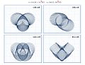
  j=3 k=4
  

  
  


• 
  

  

  
  

  
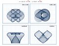
  j=3 k=4
  

  
  


• 
  

  

  
  

  
  j=3 k=4
  

  
  

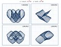
x=icos⁡(at)−cos⁡(bt)sin⁡(ct)y=jsin⁡(dt)−sin⁡(et){displaystyle {begin{aligned}x&=icos(at)-cos(bt)sin(ct)\y&=jsin(dt)-sin(et)end{aligned}}}

• 
  

  

  
  

  
  i=1 j=2
  

  
  

Examples in three dimensions

Helix

Parametric helix

Parametric equations are convenient for describing curves in higher-dimensional spaces. For example:

x=acos⁡(t)y=asin⁡(t)z=bt{displaystyle {begin{aligned}x&=acos(t)\y&=asin(t)\z&=bt,end{aligned}}}

describes a three-dimensional curve, the helix, with a radius of a and rising by 2πb units per turn. Note that the equations are identical in the plane to those for a circle.
Such expressions as the one above are commonly written as

r(t)=(x(t),y(t),z(t))=(acos⁡(t),asin⁡(t),bt),{displaystyle mathbf {r} (t)=(x(t),y(t),z(t))=(acos(t),asin(t),bt),}

where r is a three-dimensional vector.

Parametric surfaces

A torus with major radius R and minor radius r may be defined parametrically as

x=cos⁡[t][R+rcos⁡(u)],y=sin⁡[t][R+rcos⁡(u)],z=rsin⁡[u].{displaystyle {begin{aligned}x&=cos[t]left[R+rcos(u)right],\y&=sin[t]left[R+rcos(u)right],\z&=rsin[u].end{aligned}}}

where the two parameters t and u both vary between 0 and 2π.

• 
  

  

  
  

  
  

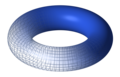
  R=2, r=1/2
  

  
  

  
  

As u varies from 0 to 2π the point on the surface moves about a short circle passing through the hole in the torus. As t varies from 0 to 2π the point on the surface moves about a long circle around the hole in the torus.

Examples with vectors

The parametric equation of the line through the point (x0,y0,z0){displaystyle left(x_{0},y_{0},z_{0}right)} and parallel to the vector ai→+bj→+ck→{displaystyle a{vec {i}}+b{vec {j}}+c{vec {k}}} is^[7]

x=x0+a⋅ty=y0+b⋅tz=z0+c⋅t{displaystyle {begin{aligned}x&=x_{0}+acdot t\y&=y_{0}+bcdot t\z&=z_{0}+ccdot tend{aligned}}}

See also

• Curve


• Parametric estimating


• Position vector


• Vector-valued function


• Parametrization by arc length


• Parametric derivative

Notes

External links

• 
  Graphing Software at Curlie
  


• Web application to draw parametric curves on the plane